Optical flow models tend to look great on the “average case,” then quietly fall apart in exactly the situations you care about: fast egomotion, compound object motion, heavy occlusion, and optics that don’t behave like a pinhole camera. The frustrating part is that many popular benchmarks don’t let you isolate those failure modes. Real-world datasets are realistic but hard to control, while synthetic datasets are scalable but often mix motion types together in a way that makes analysis fuzzy.
This project started from a simple question: if optical flow is fundamentally the interaction of camera motion, object motion, and visibility, why aren’t we evaluating models along those axes? We built a scenario-based dataset generator by extending Kubric’s simulation pipeline (Blender + PyBullet under the hood) and wrapping it with a configuration layer that can systematically enumerate motion scenarios. The end result is not just “more synthetic data,” but a structured test space you can use to diagnose, benchmark, and fine-tune models with intent.
The key idea: factorize motion scenarios
Instead of sampling random scenes and hoping rare cases show up, the generator treats a “scenario” as a product of a few controllable dimensions: camera trajectory (fixed, linear translation, rotation, or a smooth path), object motion (static, sliding, rotating), object count (up to three), and a set of imaging challenges (bar occlusion, fisheye distortion, raindrops). That framing turns evaluation into something you can reason about: if a model fails, you can say what it failed on, not just that it failed “sometimes.”
What the simulator produces
Every run outputs short, multi-object videos with dense supervision. Each sequence is 23 frames long (so you get 22 consecutive frame pairs), and the renderer exports perfect ground truth forward optical flow along with depth and masks. We kept the default resolution at 256×256 on purpose: it’s high enough to preserve motion boundaries and occlusion structure, but cheap enough that you can sweep dozens of scenario combinations without turning the project into a compute budget exercise.
To make the “imaging effects” dimension feel tangible (and not like an afterthought), we implemented effects that change the actual rendering physics rather than painting noise on top. In the team, my contribution focused on adding the lens-and-occlusion layers: fisheye distortion, raindrops, and the deterministic bar blocker.
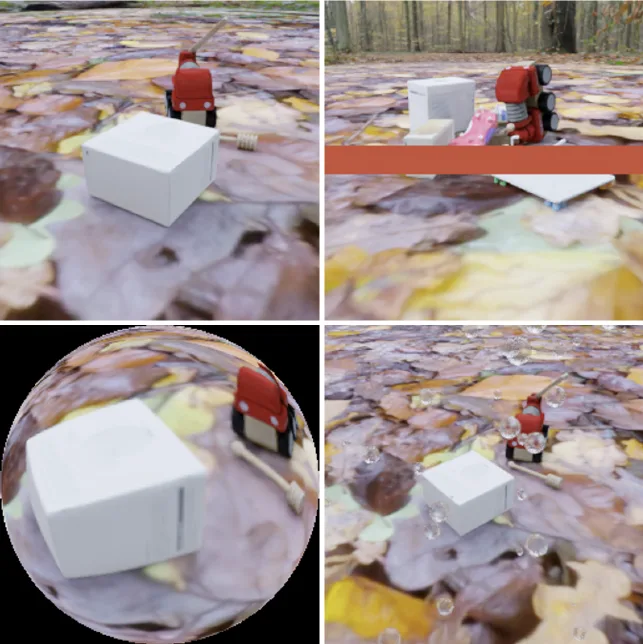
The clean render is the baseline. The bar occlusion is intentionally blunt: it creates a predictable missing region so you can stress-test correspondence reasoning without depending on brittle physical occluders. The fisheye render introduces non-linear distortion that breaks the assumptions many pipelines implicitly rely on. The raindrop render is generated through Blender’s geometry and shader graph so drops refract, occlude, and interact with lighting in a way that actually changes pixel correspondences.
How the system is organized
We structured the pipeline so experiments are defined by configuration rather than code edits. Hydra drives reproducible parameter sweeps; the scenario generator instantiates a Kubric scene with the requested camera and object motions; Blender renders frames and annotations; and a small post-process step organizes outputs into train/test splits with stable naming so models can be evaluated by scenario category.
That separation is what makes the system useful as an engine. You can say “give me camera rotation with sliding objects, object count three, with bar occlusion” and get a dataset slice that matches that description, then swap one knob at a time to see what really changed.
Three engineering pieces that mattered
Camera motion is the first place “random” becomes useless. We implemented camera trajectories that are analyzable and reproducible: linear motion with fixed orientation, rotation around the scene, and smooth path-following driven by Bézier interpolation (with optional path import). This is what lets you create compound motions on demand instead of relying on whatever the simulator happens to produce.
For weather, we avoided image-space overlays and treated rain as part of the scene. Using geometry nodes, each raindrop is a 3D element with a water-like material, so it introduces both occlusion and refraction. This matters for optical flow because the “hard parts” aren’t just noise—they’re ambiguous correspondences and distorted motion boundaries.
For occlusion, we added a deterministic, texture-based bar blocker. It’s deliberately simple and cheap, but it’s also exactly controllable. That makes it a practical tool for leave-one-category-out tests where you want to exclude an occlusion type from training and then measure whether a model learns to generalize anyway.
What it looks like in supervision space
The flow fields make the dataset’s intent obvious: the same scene can go from “clean and easy” to “ambiguous and occluded” without changing the underlying motion scenario.
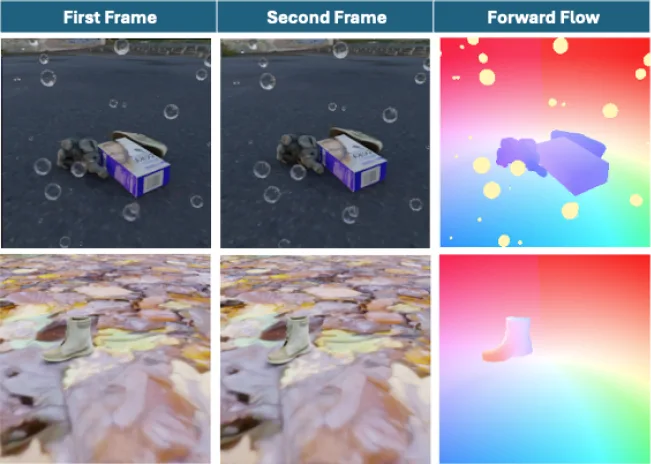
In the raindrop case, parts of the scene become partially unreadable, and the flow map reflects that complexity at boundaries and around occlusions. In the cleaner case, motion is easier to follow and the flow stays smoother. Having both under the same scenario taxonomy is what lets you separate “the model can’t handle rotation” from “the model can’t handle occlusion layered on top of rotation.”
Outcome: targeted evaluation, not just a leaderboard number
Using the generated dataset, we evaluated a range of optical flow architectures and found a consistent pattern: earlier CNN baselines struggle once you introduce rotation-heavy camera motion or compound motion with occlusion, while more modern architectures such as RAFT and FlowFormer hold up better and benefit more predictably from targeted fine-tuning. The most reliably difficult corner case was camera rotation combined with occlusion, which matches the intuition that long-range correspondence plus missing regions is where local cues stop being enough.
This work is described in the CVIU preprint “Customizable Motion Scenario-based Dataset Generation for Optical Flow Evaluation” (Hooshyaripour, Liao, Lang, Neumann, Petriu). The code for the generator and dataset organization is open sourced on GitHub at the link above.
If we extended this further
The next natural direction is to expand beyond rigid motion: articulated/deformable objects, rolling shutter, and more domain randomization in materials and lighting, while keeping the same scenario-first organization. The goal would stay the same: make “stress-testing optical flow” something you can do deliberately, not something you hope happens when you download a big dataset.